Usage Instructions

This section explains the most important steps to calculate the traction forces for an image. For a detailed explanation of all the fields, see Section 4. Save the progress at any time during this process by clicking File > Save or the floppy disk icon.

Loading Image

The mouse navigates in the user interface (UI). Right click and drag moves the field of view. The mouse wheel zooms in and out. When Cellogram starts up there is no image loaded. First, click on the Load Image in the UI or select File > Load Image (Figure 1: Stage 1 - Detection). Navigate to a grayscale image in Portable Network Graphics (png) or Tagged Image File Format (tiff) format and select and load the image. The image should appear as seen in the screenshot in Figure 1.

Figure 1. Stage 1 - Detection.

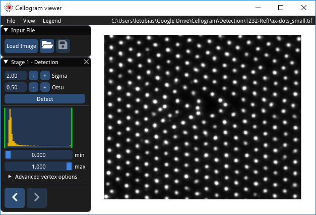
Marker Detection

For the detection of the markers Gaussian are fitted in the image. The fields under Stage 1 - Detection are Sigma which determines the size of the Gaussian that are fitted. A good starting value for is 1.5 and 3 for QDs and pillars, respectively. This value may need to adjusted depending on magnification and marker size. To start detection click on the Detect button. In case markers are missed, or detected incorrectly they can be added or deleted under Advanced vertex options or with the hot-keys a and d.

Reference Estimation

The connectivity of the mesh is found by clicking on the right arrow button in Stage 1 - Detection menu (Figure 1). If the meshing step finds missing or surplus markers, it fixes them. Removed markers are marked orange, while added markers are green. Should there be added marker, the user has the option to move the added marker to the correct position by clicking Move vertex in the Stage 2 - Meshing menu before proceeding. Next click on the right arrow button to relax the mesh and find the reference position. The displacements become visible (Figure 2).

Figure 2. Stage 3 - Analysis.

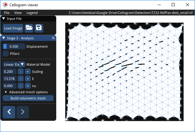
Finite Element Analysis

For the finite element analysis (FEA) enter the material parameters in the Stage 3 - Analysis menu. Hover the fields to get information on the individual fields and units. Next click Build volumetric mesh to generate a finer mesh for the analysis (Figure 2). The density of the mesh is tuned in the Advanced mesh option see Section 4 for details. Once the mesh is available, click the right arrow button to start the FEA.

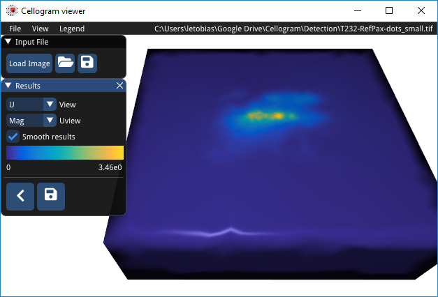
Results

Once the FEA is complete and the Results menu is visible (Figure 3). At this point the process is complete but the viewer has options to either show the displacements U or the tractions T.

Figure 3. Results.